Research So Far
Overview
This is my first post so I’m going to summarize what I’ve done this year and what my plans are for the near future.
I spent the spring semester mostly taking taking classes. When I had time I worked on learning C++, expanding my Bash scripting skills, and building a repo for my dotfiles1. This summer I’ve been learning about numerical hydrodynamics and how to implement a code that solves the Euler equations in 1D using second-order Gudonov methods.
Learning C++
I mostly learned C++ using Kate Gregory’s Pluralsight class on basic C++ supplemented with “Accelerated C++: Practical Programming by Example” by Koenig and Moo. Kate Gregory’s class was ok, it wasn’t really broad or in depth enough for what I needed and was clearly directed at computer scientists does “medium” performance computing, i.e. game development and the like. “Accelerated C++” was a better learning tool but it is not for beginner programmers; it is suitable for someone who is an intermediate program but isn’t familiar with C++.
I ended up choosing Visual Studio Code as my IDE for C++ development since no other IDE supported C++, CUDA, and HIP; plus the extensibility of VSCode is a huge plus. The GPGPU support in VSCode is pretty lacluster but it does work well for developing on remote machines which is a huge plus.
As a part of this I also learned how to use Doxygen for C++ code documentation. It’s excellent and I’ve been using it for all my projects.
Cholla
On and off throughout the spring and early summer I got Cholla up and running on Pitts H2P cluster. This was a good way to refresh on using batch systems and I found a bug in how Cholla chooses whether to use 32 or 64 bit floats. My fix unfortunately broke some other stuff and it’s almost never run with 32 bit floats so we’re ignoring that for now. I did submit a pull request to fix a bunch of typos and a few similar errors. I plan on working more on Cholla once I’m ready to start implementing magnetohydrodynamics (MHD) later this year or early next.
I also attended the OLCF new users workshop and it was very useful.
Hydrodynamics and Simulations
This was my first real dive into numerical simlation and took up the bulk of my summer. My past programming has all been data analysis of some variate so as you might expect I have a lot to learn. I started by reading the first several chapters (up to the end basic Gudonov methods) in “Computational Gas Dynamics” by Laney, “Introduction to Computational Astrophysical Hydrodynamics” by Zingale, and “Riemann Solvers and Numerical Methods for Fluid Dynamics” by Toro; I mostly followed along with Zingale since it was the easiest to follow. During this time I wrote programs to solve the Advection and Burgers equations as a stepping stone to a full Euler equations solver. These simplier, single equation solvers were a great way to start learning about numerical simulations and my implementations of them can be found in the basic-solvers directory of my hydro-sandbox repo. They are solved using second order in both space and time and use Minmod or MC slope limiters
Writing a full solver for the Euler equations was a much larger endeavour. This solver is basically made up of two parts: one that computes the slopes, time steps, reconstructs interface states, etc and a Riemann solver. My first step was writing the Riemann solver, instead of using an approximate solver I implemented the exact Riemann solver from Toro. This exact Riemann solver is used to determine the state of a hydrodynamics system that has a discontinuity in it, much like you find at each cell interface. Unfortunately the exact Riemann solver is fairly complicated so I took about a week and make a flowchart of it in ( \latex ). This helped clarify it to me and made it far easier for me to implement the Riemann solver.
Once the Riemann solver was written and tested it was time to write the whole simulation code for the Euler equations. I decided to implement this using an object oriented paradigm since I need practice with that and this algorithm is a good candidate for object oriented programming (OOP); due to the many functions that can (and should) be hidden from the main function. I wrote one class for the Riemann solver, one for the grid, and one for the simulation itself. Then all the main function has to do is call various methods of the simulation class. This general idea worked very well however I had to do large refactors, nearly rewrites, twice. Once because I was storing everything as primitive variables (density, velocity, and pressure) instead of conserved variables (density, momentum, and energy), this is a problem because it makes the conservative update hard and it doesn’t extend well to MHD. The second rewrite was because I was iteration over cell interfaces and computing the updates one cell at a time. This doesn’t work because you end up computing the same flux multiple times, this is both inefficient and can lead to numerical instability. After these refactors the code was significantly easier to read and understand. Between the complexity of the code, the multiple refactors, and hunting tricky bugs this took me about two months to do. During the debugging phase of this project I also learned how to use GDB to debug C++ code and how to hook it into VSCode. The details of the Euler solver can be found in the euler-solver directory of my hydro-sandbox repo.
As a part of writing this code I also wrote some python programs to generate animations of the output of the various solvers I wrote. These scripts used the matplotlib.animate library and were invaluable in diagnosing errors and presenting my work and a gallery of them is at the end of this post. They can be found in the visualization directory of my hydro-sandbox repo.
Miscellanous Other Projects
- Put together a personal website and research blog
- Wrote a CV and update my resume
- Attended department workshops on python, numpy, and visualizations
- Attended Oakridge National Lab’s (ORNL) OLCF new users training, i.e. how to use ORNL’s computing resources
Gallery of Results from Hydrodynamics Codes
If you’re having trouble viewing these videos try opening them in a different tab
Advection Equation
Here’s the result of solving the Advection equation with a step function initial conditions. Note the little “ears” on the profile, this is caused by the unlimited slopes that are being used.
This is the same advection simulations but now with MC limiting. Notice how the “ears” are completely gone and the profile much more resembles the initial profile, just advected to the right.
Burgers Equation
In these animations you will see the solution to the Burgers’ Equation with sinusoidal initial conditions and different slope limiters. The first is with MC limiting, this can be considered the fiducial result
Now we create the same plot but with just a forward difference. Note the oscillations near the back of the sign wave
Now we create the same plot but with just a backward difference. Note the oscillations near the front of the sign wave
And finally with a centered difference. Even though a centered difference is technically second order accurate you can see how important limiting is to getting a physically realizable result
Euler’s Equations
Now here are the results for the full Euler Equations solver.
The first animation shows a simply advecting density wave using a piecewise constant method to reconstruct the interface states. Note how quickly the profile goes from a step function to a gaussian and then how quickly it dissipates.
This is the same initial conditions but now we’re using Zingales piecewise linear method with MC limited slopes. Now how much less dissipative the advection is.
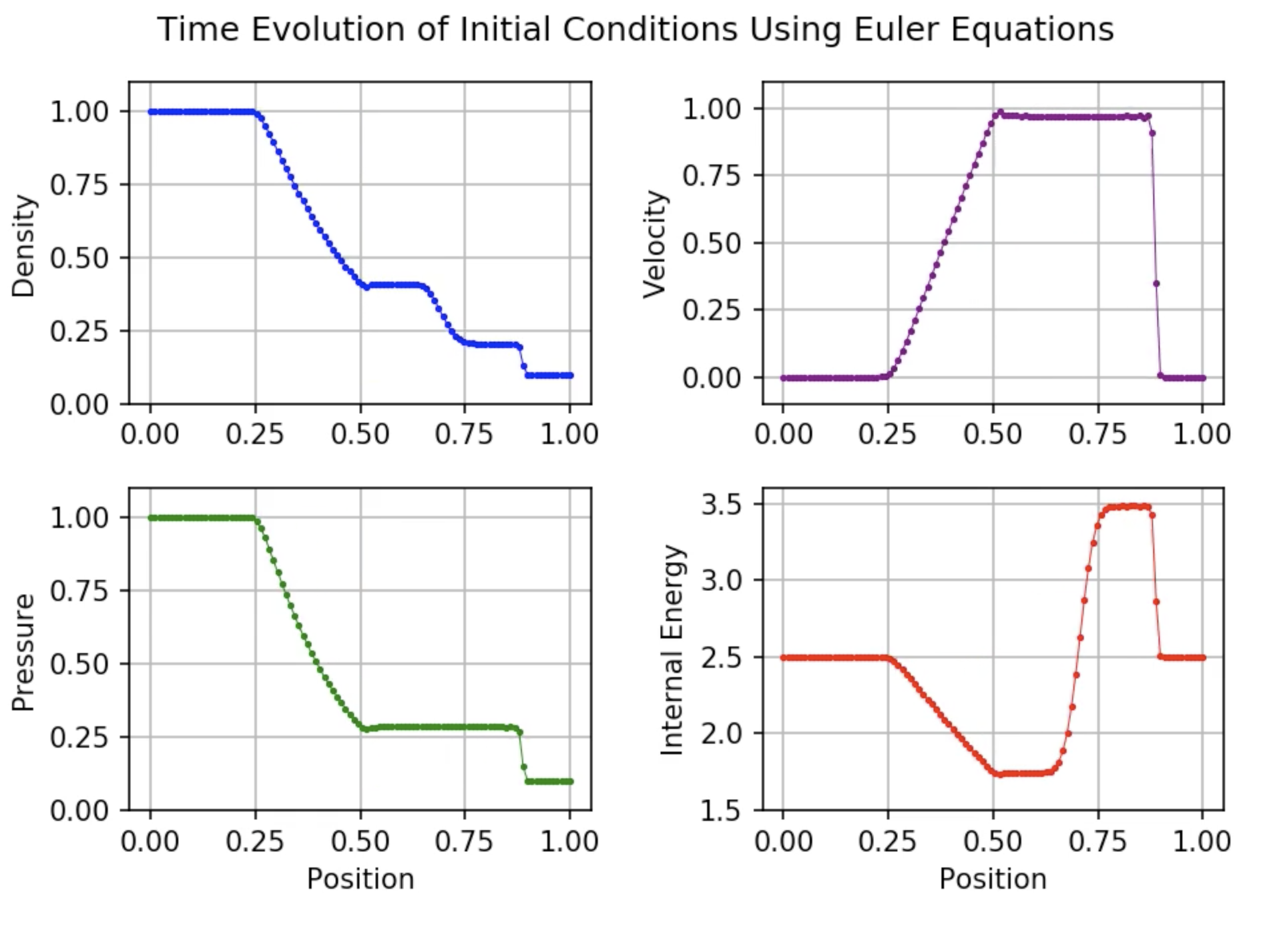
Finally the standard test of any Euler solving code, the Sod shock tube. The code reproduces the correct profile with only very small deviations, and this is with only 100 cells. With more cells it’s even more accurate