Iseult Visualization Code
Project Summary
My first project as an RSE at Princeton was to work on the Iseult visualization code adding some new features and fixing up some outstanding bugs. In total my work encompasses about 3,300 changes across 17 PRs, I won’t list everything here but will discuss some of the more significant changes.
Best Practices
The code hadn’t been maintained in awhile so I made some changes to update it to support newer versions of Python and the libraries that Iseult uses. The only significant issue that popped up was that Iseult uses some Matplotlib protected member variables and the format and usage of those variables changed in Matplotlib v3.8. Trying to fix this rapidly spiralled into greater and greater complexity and my time on this project was limited so as a workaround I created a conda environment that has the proper version of Matplotlib for Iseult. The conda environment is defined in the environment.yml file in the Iseult repo root. More details can be found in this comment in Issue #15.
I also added tests for most of the new code I was adding and setup GitHub Actions to run the tests on every PR.
Tristan v2 Data
Originally Iseult could only read data from Tristan v1 and a major part of this project was enabling Iseult to read in data from Tristan v2 as well. Originally all the data accesses were hard coded and didn’t have the flexibility to add new data formats easily. I converted all the file paths to use the Pathlib library and wrote a function that takes the path, dataset name, and a few other arguments. This function then verifies the file exists, determines the format, and loads the data with any transformations required to put it into Tristan v1 format so that the rest of the code does not need any significant changes. It should be reasonably easy to extend to other Particle-In-Cell datasets, though only Tristan v1 and v2 are supported at the moment.
Magnetic Streamlines
The other major portion was adding the ability to overlay magnetic streamlines onto several of the plot types in Iseult. I compared a two options for doing this, the matplotlib.pyplot.streamplot function and the method described on Patrick Crumley’s (the original author of Iseult) blog. I ended up deciding to use the matplotlib version because they had similar performance and matplotlib made prettier and more customizable plots more easily. Performance was a major concern, both methods took 10-30 seconds to make a streamline plot on typical datasets which would cause an unacceptable amount of lag when using Iseult. The solution I used for this was to subsample the magnetic field data with a simple stride, i.e. simply taking every Nth value. This resulted in a ~100x speedup (~200-300ms to generate a plot) when using a stride of 10 and the resulting plot was nearly visually identical to the full resolution version; see example below. The density of streamlines also had a significant, though lesser, impact on performance. I added both the stride and the streamline density as options that the user can change if they want higher density/more accurate streamlines at the cost of taking longer to generate plots.
To illustrate the impact of stride on the streamlines, below are two density plots with the magnetic streamlines overlaid on them. The first plot uses a stride of 1 (i.e. no subsampling) for the streamlines and the second uses the default stride of 10. While there are some differences, the differences are very minor and don’t change the qualitative results at all.
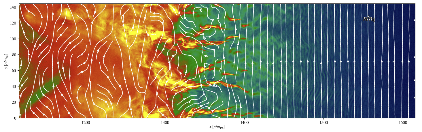 An example of a plot with the streamline overlay in Iseult with the stride set to 1
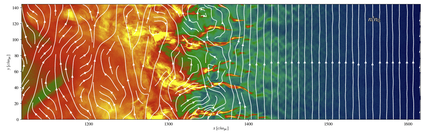 An example of a plot with the streamline overlay in Iseult with the stride set to 10, the default